
Social Network Analysis for Computer Scientists
This course deals with computer science (CS) aspects of social network analysis (SNA), and is open to all students in the master computer science programme at Leiden University.
Course information
Lectures: Fridays from 9:00 to 10:45 in Gorlaeus lecture room CM 1.26
Lab sessions: Fridays from 11:00 to 12:45 in Gorlaeus lab rooms DM0.09, DM0.13 and DM0.21
Prerequisites: a bachelor degree in CS with courses on Algorithms, Data Structures, and, Machine Learning or Data Mining
Literature: The Atlas for the Aspiring Network Scientist (by Michele Coscia, v3, 2025)
Examination: assignments throughout the semester and a final exam at the end of the semester
Brightspace link:
2627-S1 Social Network Analysis for Computer Scientists
Study guide link: Social Network Analysis for Computer Scientists
Study points: 6 ECTS
Course staff: prof. dr. Frank Takes (f.w.takes@liacs.leidenuniv.nl, BE 3.07),
Rachel de Jong MSc (BE 3.03)
Assistants:
Gamal Adel Elgamal MSc (BE 3.23),
Nicholas Assiotis BSc, Agata Cieliczko BSc, Bart Holterman BSc, Rachel Hau BSc and Mark Wijnands BSc
![[Network visualization image]](yeast_eccs.jpg)
Network with 1458 nodes and 1948 edges.
Course schedule
| Date | Lecture (9:00-10:45) | Lab session (11:00-12:45) | |
| 1. | Fri Sep 4, 2026 |
Lecture 0: Course information (Chapter 1) Lecture 1: Introduction to network analysis (Chapter 6, 8 and 10) |
Instruction: Introduction to Gephi Work on Assignment 1 |
| 2. | Fri Sep 11, 2026 |
Lecture 2: Small world phenomenon, Advanced network concepts and Centrality (Chapter 7, 12, 13 and 14) |
Instruction: Introduction to NetworkX Work on Assignment 1 |
| 3. | Fri Sep 18, 2026 |
Lecture 3: Applied network concepts and Network projection (Chapter 9, 26.1, 30 and 31) |
First ANS Practice Session Work on Assignment 1 |
| 4. | Fri Sep 25, 2026 | Lecture 4: Community detection and Core/periphery structure |
Work on Assignment 1 |
| 5. | Fri Oct 2, 2026 | Lecture 5: Structure of the web and propagation-based centrality |
Work on Assignment 1 |
| Mon Oct 5, 2026 | Deadline for Assignment 1 (14:00; hand in via Brightspace) | ||
| ... | ... | ... | ... |
| Mon Nov 9, 2026 | Deadline for Assignment 2 (14:00; hand in via Brightspace) | ||
| ... | ... | ... | ... |
| Fri Dec 11, 2026 | Exam (in USC) | ||
| Mon Dec 14, 2026 | Deadline for Retake Assignment to replace failed assignment(s) (14:00; hand in via Brightspace on top of failed assignment) | ||
| Thu Dec 17, 2026 | Exam result inspection opportunity (12:00 in teacher's office BE 3.07) | ||
| Jan 29, 2027 | Retake Exam (in USC) | ||
The main goal of this session is to get to know the ANS system for digital examination, and practice with more theoretical aspects of the course.
Navigate to ANS, and follow the instructions there.

The main goal of this lab session is to become familiar with
NetworkX (a Python package to analyze networks for research purposes).
All relevant information on NetworkX can be found in the NetworkX online documentation.
Your Python environment
For this lab session, you need a working Python environment. For this, there are two options:
- Use your own self-installed Python environment, and choose your own editor and way of running code (via the command line, an IDE or an interactive notebook). Proceed to Instructions for today
- Alternatively, you can use the desktop machines in the student computer rooms. One easy way to create a Python environment on the university computers, is to use conda. As of 2024, conda appears to be installed already. Therefore, you can likely skip step 1--3 below, and start at step 4.
- Download Miniconda by running the following command in your terminal:
wget https://repo.anaconda.com/miniconda/Miniconda3-latest-Linux-x86_64.sh - Install Miniconda:
bash Miniconda3-latest-Linux-x86_64.sh
The installer will ask you some questions. Normally, the standard location suffices and you do not have to add conda to PATH. - After installation finishes, close your terminal so that the changes take effect.
Upon opening a new terminal, activate the conda virtual
environment with:
source miniconda3/bin/activate
If all goes well, you will see that (base) appears in front of your shell prompt. This means that conda's base environment is active.
- Create a new conda environment:
conda create --name snacs
And activate it with:
conda activate snacs
You might use conda for other courses as well, and version conflicts can arise when you install many packages. Using separate environments prevents this.
NOTE: some packages can make your conda environment take up a lot of space. So try not to use an unnecessary number of environments with duplicate packages. You can also remove an environment that you don't need anymore, see the conda cheatsheet. - Packages can easily be installed with conda. To install NetworkX, run:
conda install networkx -
Getting started
- Running code from the command line. Now you should be able to run your code from the command line by typing
python3 scriptname.py -
Running code in interactive Jupyter notebook from the university environment:
conda install -c conda-forge jupyterlab
After installing that once, the notebook/lab can be started using:
jupyter lab
(When using Jupyter through SSH, so when it is not running on the machine that you are currently working on, make sure to use port forwarding whilst SSH-ing, using options -g -L 8888:127.0.0.1:8888. Also add options --no-browser and --port=8888 when starting up Jupyter.)
- Running code from the command line. Now you should be able to run your code from the command line by typing
Instructions for today: Lab session on NetworkX
- Take some time to do the NetworkX tutorial.
- Have a look at functionality to read and write graphs from/to disk, and in particular learn how to import an edge list. Understand the input format and ways of including things like Weight and other attributes of edges.
- A lot of the common network metrics you may want to compute are implemented as NetworkX function or NetworkX algorithm. Become familiar with these, for example by computing measures such as degree assortativity, clustering, density, diameter and average distance.
- While at it, why not take a look at how NetworkX relates to other data formats?
- Try to load the network from the first lab session (small-gephiready.tsv) into NetworkX, and investigate some characteristic properties of the network, such as the degree distribution and distance distribution. Use theread_edgelist function and remember to select the correct separator (tab), and pay attention to the header of the file.
- Get the Epinions network from the SNAP repository. You may need to fiddle with the precise header, but it is already in edge list format. Compute some common characteristics such as the degree distribution, and visualize them using appropriate figures or distributions, for example using pyplot/Matplotlib.
- What are the differences between NetworkX and Gephi in terms of visualization and analysis capabilities?
Done? Proceed with Exercise 2 of Assignment 1.
Looking for a challenge? Check out these three alternatives (that you
can also use instead of NetworkX throughout the course, if you prefer
(but for which there is less help available)):
- Python igraph, a Python version of the R igraph package.
- Graph-Tool, a python graph analysis toolkit that leaves the hard computation to parallel (OpenMP) C++ code.
- SNAP, which is entirely written in C++ and has many interesting features. Nowadays, there is also a Python version.
Running intro problems regarding prior knowledge on python programming? See the reading material at the bottom of this course website.
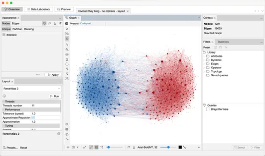
About social network analysis tools and packages. There exist different tools and packages for social network analysis. In this course, we cover two of them, with complementary advantages:
- Gephi, an easy-to-use tool with a graphical interface useful for visualization
and quick analysis of relatively small network data (this week, see below).
- NetworkX, an extensive Python package for network analysis that can handle larger network datasets and computations (next week).
Learning goals. The main goal of this lab session is to become familiar with Gephi (experimental beta-software to visualize networks for research purposes) and its input format. At the end of this session you should be able to:
- Know how to use Gephi for social network analysis
- Import and visualize raw network data with labeled nodes and labeled and/or weighted edges (directed or undirected),
- Understand how to map edge and node size and color to structural network properties such as the node degree and edge type,
- Know how to apply filters to the visualization, for example to focus only on the giant component,
- Export a vector graphic PDF of your network for reuse in for example a presentation or paper,
- Export computed node data for reuse in another program.
There is no deliverable for this lab session, but you are assumed to know the tool afterwards. Practice more at home if needed.
Instructions for today: Walk through the complete Gephi tutorial.
Note that the tutorial briefly covers topics such as centrality and communities, which will not be covered extensively until Lecture 2, 3 and 4.
Done? Get started with the practical part of Assignment 1. You can download the datafiles here. If you want to analyze huge.tsv, you will have to get it from the shared folder in the ISSC Linux or LIACS DS lab environment, as stated in the assignment.
Reading material
In the past, students have expressed interest in additional reading material to help freshen up on skills and knowledge required for this course.
- To brush up on your Python programming skills, you could do Lecture 0, 1 and 4 of these Scientific Python Lectures.
- To freshen up your LaTeX skills, you could do for example this LaTeX tutorial by Overleaf.
- MIT
hashad (sorry, the URL is broken) a nice online course on discrete mathematics. Relevant chapters: 5, 6 and 7. - The (Dutch) Leiden courses Algoritmiek (Algorithms) and Datastructuren (Data structures) might also be interesting to browse through.
- Basic knowledge of concepts in machine learning and data mining is provided, e.g., at the Wikipedia machine learning page.