Artist Recognition With Convolutional Recurrent Neural Networks
API 2017 / 2018 Project Site
Joost Nibbeling - s1253727
1. Introduction
Deep convolutional neural networks have been successfully applied to many tasks. Chiefly among those have been image and video classification or recognition related tasks. But convolutional neural networks have also been successfully applied for speech recognition and even music classification [1].
For audio related tasks, the raw audio is usually converted to a time-frequency representation such as Mel-spectograms. This is then supplied as input for some neural network. Choosing and creating the correct representation however, requires the right domain knowledge. Therefore, it would be helpful if this could be skipped, and audio could be directly fed into a convolutional network. This way less domain knowledge would be required to create an effective neural network.
[2] proposes deep convolutional models that performs convolutions on a small number of samples in the range of 2 to 5 samples at a time. These networks were used for music auto-tagging. For this project these models have been extended with a recurrent layer. These models are then used for artist recognition instead of auto-tagging.
In this paper these convolutional recurrent neural networks are described in detail. Experiments with this network have been performed on the MagnaTagATune dataset for different parameters. The question is how well do these recurrent convolutional models perform on their own and when compared against the original convolutional models for the task of artist recognition. The impact on musical on prediction accuracy is also evaluated.
2. Model
The models used are based on the ones that worked best in [2]. In this paper, the models were build out of standard building blocks that consist of a convolutional layer with a filter size of n followed by a max-pooling layer with a pool-size of n. The convolutional layer in these block is padded so the output has the same size as the input. Therefore, after each of these blocks, the input size is reduced by a factor of n.
The input layer is also a convolutional layer. This layer performs directly on the raw audio samples. This is a strided convolutional layer with the stride equal to the filter size. So, this first layer reduces the input by a factor equal to the filter size. The best results are obtained when this layer works on a small number of sample. Therefore, the filter size of this layer should be small.
These blocks are than combined in such a way that after all the standard building blocks the input has been reduced to size 1. For this project, the best configuration found by [2] is used. This configuration is n = 3, and a filter size and stride of 3 for the initial convolutional layer. This means the input needs to be a power of 3. This configuration is shown schematically in table 1. A concrete example of a possible model is shown in table 2.
| Table 1. Original model, m is # standard blocks | ||
|---|---|---|
| Input size = 3m+1 | ||
| Layer | Configuration | Output |
| Convolutional layer | Size = 3, Stride = 3 | 3m |
| Repeat m times the standard building block | ||
| Convolutional layer Max-Pooling layer | Size = 3, Stride = 1 Pool size = 3 | 3m-1 |
| After m repetitions | 30 = 1 * number of filters last building block | |
| Fully Connected layer | - | Number of nodes |
| Output layer | - | Number of classes |
A concrete example of a possible model is shown in table 2. This model takes 729 samples as input. The first strided convolutional layer cuts this input by a factor of 3 to 243 samples. Each Max-pooling layer of the standard blocks reduces the input by a factor of 3 again. To get an output size of 1 at the end, 3log(243) = 5 building blocks are necessary. Following the final block is a fully connected layer. The last layer is the output layer. In this example there would be 64 different classes.
| Table 2. Example original model | ||
|---|---|---|
| Input size = 729 | ||
| Layer | Configuration | Output |
| Convolutional layer | Size = 3, Stride = 3, Filters = 64 | 243*64 |
| Convolutional layer Max-Pooling layer | Size = 3, Stride = 1, Filters = 64 Pool size = 3 | 243*64 (padded) 81*64 |
| Convolutional layer Max-Pooling layer | Size = 3, Stride = 1, Filters = 64 Pool size = 3 | 81*64 (padded) 27*64 |
| Convolutional layer Max-Pooling layer | Size = 3, Stride = 1, Filters = 128 Pool size = 3 | 27*128 (padded) 9*128 |
| Convolutional layer Max-Pooling layer | Size = 3, Stride = 1, Filters = 128 Pool size = 3 | 9*128 (padded) 3*128 |
| Convolutional layer Max-Pooling layer | Size = 3, Stride = 1, Filters = 128 Pool size = 3 | 3*128 (padded) 1*128 |
| Fully Connected layer | Size = 128 | 128 |
| Output layer | Size = 64 | 64 |
The best results obtained in [2] are with an input size of 310 = 59049 samples and 9 building blocks. A music clip is likely to be longer than 59049 samples. In that case, it needs to be divided into segments and each segment is then classified separately. There might however, be dependencies between these different segments that these models are then unable to learn as it sees each segment individually.
Therefore, for this project the fully connected layer in the models described above is replaced with a recurrent layer. This way the convolutions can be performed on each segment individually and inputted one by one into a recurrent layer as a sequence. A recurrent layer retains a memory of previously seen elements of the sequence. If a new element is inputted into the recurrent layer, it is combined with this memory and the memory is updated. After the final element of the sequence has been inputted, a final output is generated that has considered all elements of the sequence. This way, the network may learn information about the dependencies between segments that is useful for the classification tasks, which in our case is artist recognition.
The new recurrent version is shown schematically in table 3. LSTM stands for long short-term memory and is a type of recurrent layer.| Table 3. Recurrent model, m is # standard blocks, s is # segments | ||
|---|---|---|
| Input size = s*3m+1 | ||
| Layer | Configuration | Output |
| Convolutional layer | Size = 3, Stride = 3 | s * 3m |
| Repeat m times the standard building block | ||
| Convolutional layer Max-Pooling layer | Size = 3, Stride = 1 Pool size = 3 | 3m-1 |
| After m repetitions | s * 1 * number of filters last building block | |
| LSTM layer | - | Number of nodes |
| Output layer | - | Number of classes |
A concrete example of the recurrent model can be found in table 4. In this example there are 7 segments of 729 samples. Convolutions are performed on each segment separately. These are all inputted into the LSTM layer as a sequence, after which the combined output of all segments is inputted into the output classification layer.
| Table 4. Example recurrent model | ||
|---|---|---|
| Input size = 7*729 | ||
| Layer | Configuration | Output |
| Convolutional layer | Size = 3, Stride = 3, Filters = 64 | 7*243*64 |
| Convolutional layer Max-Pooling layer | Size = 3, Stride = 1, Filters = 64 Pool size = 3 | 7*243*64 (padded) 7*81*64 |
| Convolutional layer Max-Pooling layer | Size = 3, Stride = 1, Filters = 64 Pool size = 3 | 7*81*64 (padded) 7*27*64 |
| Convolutional layer Max-Pooling layer | Size = 3, Stride = 1, Filters = 128 Pool size = 3 | 7*27*128 (padded) 7*9*128 |
| Convolutional layer Max-Pooling layer | Size = 3, Stride = 1, Filters = 128 Pool size = 3 | 7*9*128 (padded) 7*3*128 |
| Convolutional layer Max-Pooling layer | Size = 3, Stride = 1, Filters = 128 Pool size = 3 | 7*3*128 (padded) 7*1*128 |
| LSTM | Size = 128 | 128 |
| Output layer | Size = 64 | 64 |
Activation functions in each for this project have been changed for this project from the proposed version from [2]. Both the recurrent and original model use the same activation functions. For the convolutional layers this is ReLu. For the LSTM layer and fully connected layer this is Tahn and for the output layer this is softmax.
3. Experiments and Results
This section describes the dataset used, the training procedure, the experiments performed on the trained models and the results.
3.1 Dataset
Because the models have been designed to work on raw samples, a dataset with for which the actual audio is available is necessary. Therefore, the dataset chosen is the MagnaTagATune dataset for which most audio is available. This audio however is only available in mp3 format. This audio is therefore first converted to wav format.
Following this some clips are removed from the dataset. Firstly, there are some clips with no audio available, and therefore not usable for these experiments. Secondly, some clips are from songs from compilation albums. These are for example tagged with artists names like various artists and not the actual original artist. This makes them also unsuitable for these experiments and all clips identified as coming from compilation albums are removed.
This leaves 24847 clips from 222 different artists. Each clip is around 30 seconds long and contains 465984 at a sample rate of 16 kHz. This means there is around 207 hours of audio in the dataset. This data is split in two different ways in a test set and training set. The 30 second clips result from longer songs that are cut up into pieces. For the first train and test set the clips are divided in such a way that the percentage of clips from a given artist roughly corresponds in both the train and test set. This means that clips from the same song are in both test and training set. The second dataset divides the clips in such a way that the percentage of clips per artist still roughly corresponds between both training and test set, but also ensures that clips from the same song only occur in either the test or training set.
3.2 Training Procedure
All models are implemented with the Keras python library with the tensorflow backend and trained on a single GTX 1080 Ti GPU for 50 epochs. This can take between 12 to 24 hours, depending mainly on the number of segments each clip is divided into.
During training batch normalization is used before each activation function as in [2]. The Adam optimizer is used, and the loss function is set to categorical cross entropy for all models. All models are trained three different times and results reported are the average of these three runs.
3.3 Performance for different splitting of the data
The first experiment tries to measure the difference of performance of the same model between the two different ways of splitting the data as described in section 3.1. In case different sections of the same song are in both the training and test set, the performance measured may be the ability of the network to recognize a song instead of an artist. This way good results could be reported, while the model may fail to recognize the artist when it sees a completely unknown song.
The model used in this experiment is the recurrent version. Clips are cut into 7 segments of 59049 samples. Any leftover samples are discarded. Using 59049 samples mean that there are 10 convolutional layers: the first strided one, and 9 layers each followed by a max-pooling layer. The exact number of filters and nodes used in each layer can be found in table A.1 for model number 1.
The accuracy in percentage is plotted in figure 1 for both training sets and test sets. It shows that while the accuracy on both training sets is similar, recognizing artists is more difficult when it is done on completely unknown songs. The accuracy on the test set after 50 epochs on the first dataset is around 56% on average, but around 42% for the second dataset. But while there is a noticeable reduction in accuracy, it does also not completely fail. This indicates that it is indeed the artist that is being recognized instead of the song. The graph also shows that for at least the second dataset the peak accuracy is reached at epoch 42. After that the accuracy starts fluctuating. A dropping and then rising accuracy can also be observed at other place for both datasets. The first dataset however, reaches peak accuracy at epoch 50. It may therefore be possible that better results could still be achieved with further training. A good stopping point may therefore be found by creating another validation set and stopping the training when the accuracy on the validation set stops increasing for some amount of epoch.
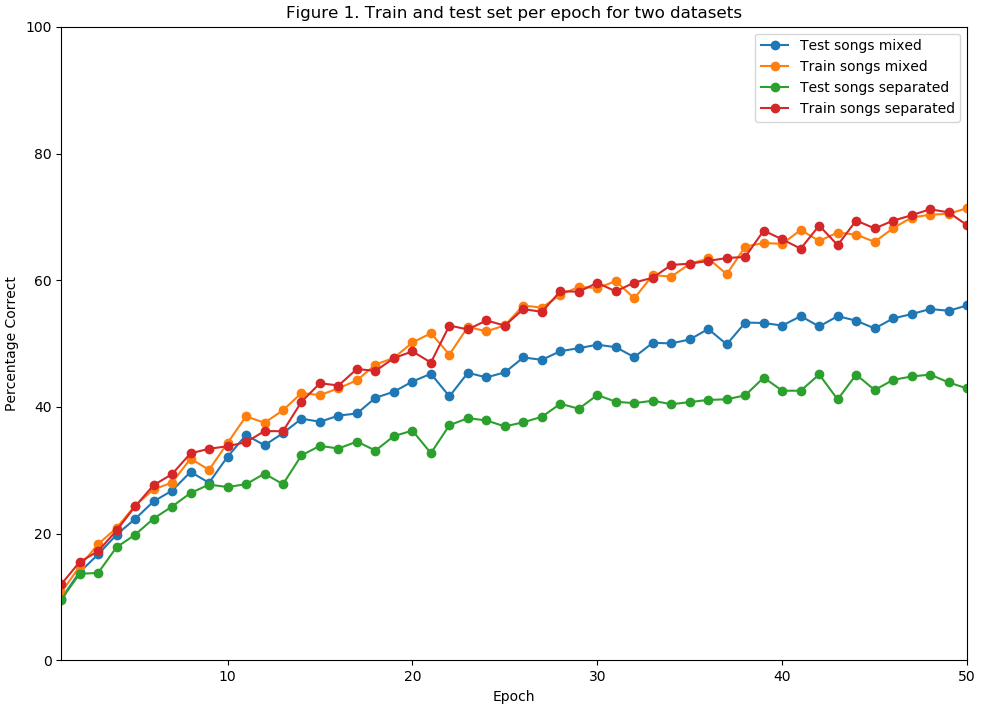
As the results show that the second dataset is the harder problem, all other experiments are performed on this dataset.
3.4 Number of filters
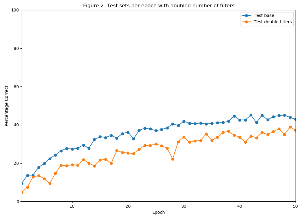
The second experiment measures the effect of the numbers of filters used. Figure 2 plots the result of two different models for the test set against the number of epochs. The first is the same one used in section 3.4. The second one is identical, except for the number of filters which have been doubled. The exact number of filters can be found in table A.1. for model 1 and 2.
The figure shows that the model with the lower number of filters consistently outperforms the other model. It is therefore important to choose this correctly to get a well performing model.
3.5 Different Segmentation Methods
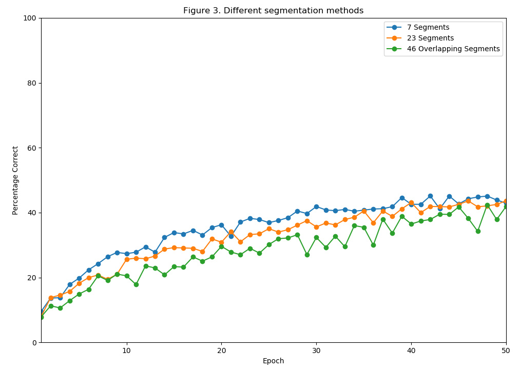
The third experiment measures the impact on performance by different segmentation methods. Three segmentation methods are used:
- 7 segments of 59049 samples. This is the same as in section 3.3 and 3.4
- 23 segments of 19683 samples. This means there are 9 convolutional layers instead of 10, but a longer sequence is inputted into the convolutional layer.
- 46 segments of 19683 samples. For clips have been cut into segments with a window of 19683 samples, but with a stride of 9841 samples. This means the last half of each segment is equal to the first half of the next segment.
The performance on the test set is plotted per epoch in figure 3. It shows that using more overlapping segments is not useful for the artist recognition, as it performs the worst. Using 7 larger segments also tends to give better performance than using smaller but more segments. This is similar to the results found by [2], where larger segments give somewhat better results.
3.6 Recurrent vs Non-Recurrent Model
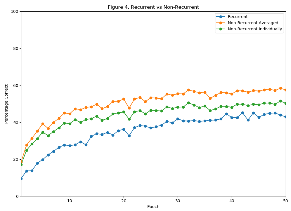
The fourth experiment is used to measure the effectiveness of the recurrent convolutional network against just a convolutional network. For the convolutional network, the recurrent layer is replaced with a dense layer as described in section 2. During training this model is trained on each segment of a clip individually. Two evaluation methods are used for this model. The first is simply predicting each segment individually. The second is averaging the predictions of all segments of a clip and using this for the final prediction. For both the recurrent and non-recurrent model, the clips are cut into 7 segments. The exact numbers of filters and nodes in the LSTM or dense layer used can be found in table A.1. for model 1. The results on the test set are plotted in figure 4.
The figure shows that the non-recurrent version works better than the recurrent version for both methods of evaluation. The point of the recurrent layer is to try and learn dependencies between segments useful for classification. It results show however, that this does not help, but only complicates the learning process. The original non-recurrent model as proposed by [2] works better for the artist recognition task.
The figure does show that there is a clear benefit in considering all segments of a clip together instead of individually. This is however better done by the simpler procedure of averaging the results afterwards, instead of trying to incorporate it into the learning process.
3.7. Top K Results
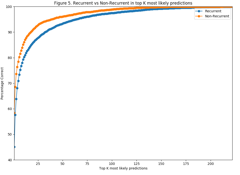
All the above results are obtained by looking at only the most likely artist predicted by the networks. It can also be useful to look at the top 2 or more predictions instead to see if the correct artist is among those. For instance, in the used dataset there are several artists that appear on their own, or in collaboration with another artist. Some results do show that the predicted artist is sometimes the artist on its own while the collaboration is the second most likely and correct prediction or vice versa. Therefore, the percentage predicted correctly on the test set when looking at the top K predictions for K = [1,222] has been plotted in figure 5. T his has been done for both the recurrent and non-recurrent version of the network. The same configurations for the models are used as in section 3.6
Initially it shows the accuracy increasing quickly when K is increased. The non-recurrent version scores around 80% for K=6. The improvements each time K is increased slow down later however. The non-recurrent version only reaches 100% for K=221 and the recurrent version only when K=222. So, the correct artist is for some clip predicted as least likely, indicating that there some clips that are very hard to predict.
3.8. Impact of Musical Genre
Finally, the impact of genre is examined. The albums in the MagnaTagATune dataset are tagged with up to three different genres from ten different possibilities. This data however, is not complete, so we have tried to complete this. As the albums are tagged and not the songs itself, the clips are assigned the genres of the album it is from. The artists are also tagged with the union of the genres of all their albums.
Table 5 shows the percentage of clips predicted incorrectly of each genre on the test set by both the recurrent and non-recurrent model. While the table shows Electronic Rock to be very difficult to predict the artist for, there are very few clips with this genre in the dataset, so this result may not be reliable. The same is true for Hip Hop. Otherwise the table shows that Jazz and Classical are the easiest to predict the correct artist for while Electro Rock is the most difficult.
| Table 5. Percentage of clips with genre predicted incorrectly | ||
|---|---|---|
| Genre | % Incorrect Recurrent | % Incorrect Non-Recurrent |
| Alt Rock | 73.38 | 50.85 |
| Electro Rock | 90.14 | 71.12 |
| Classical | 29.66 | 21.36 |
| Electronica | 65.87 | 58.05 |
| Electronic Rock | 100 | 61.05 |
| Jazz | 14.10 | 3.84 |
| New Age | 46.83 | 45.6 |
| Hip Hop | 66.67 | 50 |
| Ambient | 47.97 | 49.42 |
| World | 60.58 | 43.31 |
| Hard Rock | 56.52 | 33.54 |
It may be a reasonable idea that the predicted artist for a clip is wrong, because that artist works within the same genre. Table 6 shows the percentage of errors for which at least a single genre of the wrongly predicted clip is among the genres of the predicted artist. For both models this lies around 60%. This indicates that the genre may be a decent indicator for why the wrong artist is predicted.
| Table 6. Percentage of wrong predictions where at least one genre of the clip was in the genre of the predicted artist | |
|---|---|
| Recurrent Version | Non-Recurrent Version |
| 59.80 % | 60.63 % |
4. Conclusion and Future Work
In this paper a recurrent convolutional model is described based on the convolutional model proposed by [2]. Both the original convolutional and recurrent convolutional model work directly on raw samples, so that no further transformation of the audio is necessary. Both have been used for the task of artist recognition on the MagnaTagATune dataset. While the recurrent convolutional model works relatively well when configured correctly, the experiments also show the original convolutional model works better for this task. Experiments also show that the musical genre appears to be a factor when it comes to the correct prediction of an artist.
All experiments have been done on the relatively small MagnaTagATune dataset. Future experiments could be done to verify how well these models scale to larger datasets such as the million-song dataset. The actual audio would need to be obtained however, no just a set of extracted features. Further analysis could also be done on what exactly the learned filters learn and react to.
References
-
Hershey, Shawn, et al. "CNN architectures for large-scale audio classification."
Acoustics, Speech and Signal Processing (ICASSP), 2017 IEEE International Conference on. IEEE, 2017. -
Lee, Jongpil, et al. "Sample-level Deep Convolutional Neural Networks for Music Auto-tagging Using Raw Waveforms."
arXiv preprint arXiv:1703.01789 (2017).
Appendix
| Table A.1. Input size and number of filters / nodes all models | |||||
|---|---|---|---|---|---|
| Model | Input size | 1st # filters | Following # filters | LSTM/Dense # nodes | Output # nodes |
| 1 | 7 * 59049 | 64 |
|
512 | 222 |
| 2 | 7 * 59049 | 128 |
|
1024 | 222 |
| 3 | 23 * 19683 | 64 |
|
512 | 222 |
| 4 | 46 * 19683 | 64 |
|
512 | 222 |
Scripts and Data
In this section the information is provided to get the dataset and how to use the scripts to reproduce the experiments. Note that all scripts have been tested with a Python 2 interpreter
Download scripts and data as zip file
1. Data Preparation
1. Go here to download the MagnaTagATune dataset . Download the Clip metadata in the CSV format and the Audio Data. Unzip all the audio data.
2. The audio data is in MP3, but needs to be converted to WAV data. First the correct folder structure to store the WAV data is necessary. The shell script create_wav_folders.sh can do this. The script convert.py will do the actual conversion. It requires the pydub package. Edit the script to point it to the folder with mp3s, the folder for wavs and to the downloaded CSV file. It will also output a new CSV file that contains only the clips for which audio was available and that was successfully converted to MP3. Where this file is created can also be edited in the script.
3. Two scripts are provided to split the data in training and test sets. Both scripts make use of the numpy/scipy packages.
The script create_test_train_songs_mixed.py will create a test and training set in which clips from the same song can be in both sets.
The script create_test_train_songs_separated.py will create test and training sets in which clips from the same song will only occur in either the test or training set. Both scripts will output the test and training set as CSV files. The scripts will need to be edited so they point to the CSV file generated by the convert.py script in the previous step. Where the test and training CSV files are placed can also be edited in the scripts.
The exact splitting by these scripts is random. The exact data sets used for the experiments are also included. test_songs_mixed.csv and train_songs_mixed.csv are test and training sets in which clips from the same song occur in both sets. test_songs_separated.csv and train_songs_separated are the sets in which clips from the same song only occur in either one of them.
Recurrent Convolutional Network
All scripts in this section require:
They can be found in the recurrent convolutional network folder. Some editing of the scripts in this section will be necessary. All parameters that may need to be edited are shown at the top of the scripts and commented with an explanation. Some more information on all scripts follows below.
1. Training the network Training the network can be done with the recurrent_convolutional.py script. This script will need to be edited to point it to the training set CSV generated or downloaded in the previous section and to the folder containing the songs in WAV format. The network parameters itself can also be tweaked at the top at this script. This include how large the segmentation window should be, the stride of this window, how many epochs to train and the filter sizes and number of LSTM nodes. The batch size has a big effect on memory usage. You can try to lower it if the script crashes due to running out of memory. After every epoch the weights are saved to the disk.
2. Evaluating the network The accuracy of all epochs for the test and training set can be computed with the evaluate_recurrent_convolutional.py script. It expects the weights generated by the training script in the same folder. The script will need to be pointed to the train and test CSVs used to train the network and the songs in wav format. The network parameters can also be edited in this script and should be the same as the ones in the recurrent_convolutional.py script that computed the weights. As evaluating the training set can take a lot of time, this can be turned off. Results are also outputted in text files.
3. Generate top K results The top K accuracy on the test set can be computed for 1 specific file of weights generated by the training script with the script ktop_recurrent_convolutional.py. The script also needs to be edited to point to the test and train CSVs (train CSVs still necessary as this was used to map the artist to an index during training) and the songs in wav format. Network and segmentation parameters should again match the ones used to train the network. Results will also be stored as text file.
4. Genre Inspection To do the genre inspection on the test set, the clips tagged with genres are necessary. This is the file clips_with_genres.csv. The script to do the genre inspection is genres_recurrent_convolutional.py. This script needs to be edited to point to the clips with genres CSV, the test CSV, the same train CSV used during training, and the wav format songs. Network and segmentation parameters should again match those used during training. The script does the genre inspection on a single set of weights. Which one will also need to be edited in the script.
Convolutional Network
The scripts in this section are used in the same way and have the same requirements as all the scripts mentioned in the section above. The difference is that these scripts will train and evaluate the original pure convolutional networks instead of the recurrent convolutional networks. The scripts are:
- convolutional.py: Trains the convolutional network
- evaluate_convolutional.py: Evaluates for all epoch computed by the training script. Will output results for both averaged predictions and predictions for each segment individually
- ktop_convolutional.py: Will compute top-K results for all K on a single set of weights
- genres_convolutional.py: Will do genre inspection on a single set of weights. Requires clips_with_genres.csv